Model Predictive Control Introduction

Content

1. Introduction
2. Idea
   • Definitions
   • Optimization
   • Controller
3. Controller

Introduction.

In this post we will give a quick and shallow introduction to Model Predictive Control (MPC). This will just aim at giving an understanding of the main idea. If you want to read more on the topic there are plenty of ressources out there and ther will be some links at the end of the post. Now that this is said let’s dive into MPC.

Idea.

Definitions.

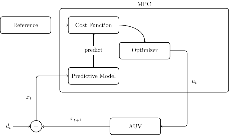
The Goal of a controller is to find a sequence of actions that will generate the desired behavior for a given agent. MPC lies in the framework of optimal control. That is it tires to control the agent in order to minimize a cost function. So lets first introduce a couple of concepts so that we are all on the same page:

• Predictive Model: This is the model used by the algorithm and serves as a proxy of the real world plant.
• Optimizer: Pretty straight forward, this is the algorithm used to find the best action.
• Cost function: This hand-designed or modeled function that is supposed to represent the deisred behavior of the agent. That is the function find it’s minimum for the optimal sequence of action. It can be parametrized by a reference the agent needs to track.

A illustration on how those elements connect is given in the following figure.

Abstract view of MPC.

Now that we have all the concepts we can give an explanation of MPC. We will try to go easy on the math but it gives a better picture of what is going on. So let \[dx \sim f(\boldsymbol{x}, \boldsymbol{u})\] be the stochastic dynamics of agent we want to control where \(\boldsymbol{x} \in \mathbb{R}^{n}\) is the state of the agent and \(\boldsymbol{u} \in \mathbb{R}^M\) is the input sent to the agent. That means that callling this function with some given state-input pair tells us how the agent will evole over time. The function is non-deterministic as there usually is some random noise fed into a real world plant.

Assume that \[ dx \sim \hat{f}(\boldsymbol{x}, \boldsymbol{u}) \] the predictive model is closely modelling the real dynamics, \(\hat{f}(\cdot, \cdot) \approx f(\cdot, \cdot)\), in the domain where the agent is working. Then we can use this predictive model as proxy for the agent and predict the agent’s behavior with it.

Finally let \(\boldsymbol{U} \in \mathbb{R}^{M \times \tau}\) be the Action sequence.

We can now recursively apply the action sequence to th predictive model to generate a tracjectory \(\boldsymbol{H} \in \mathbb{R}^{N \times \tau}\).

Examples:

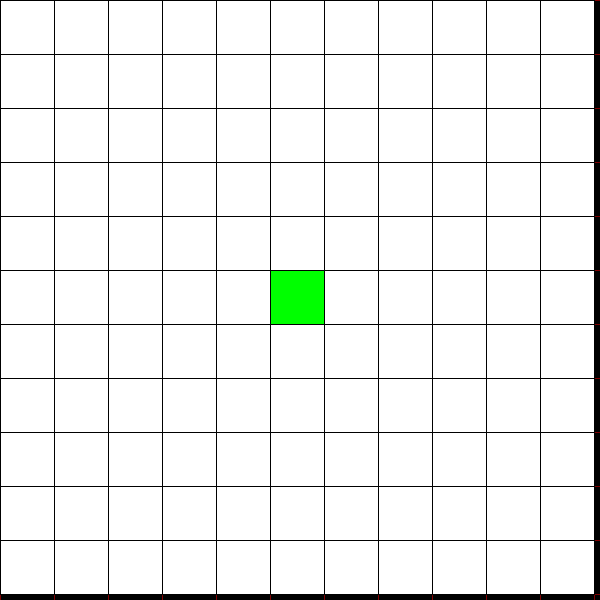
Consider the discrete deterministic action-state environment illustrated in the next figure where the inital state is the green square. Let \(\boldsymbol{u} = \{up,\, down,\, left,\, right\}\) be the avaialable actions and the state \(\boldsymbol{x} = (i, j)\) the two indexes defining the position on the space.

Envrironement

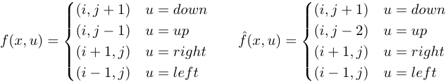
The dynamics and the predictive model are given by the following discrete functions:

Dyamics and model functions.

Assume that you have the following action sequence: \(\boldsymbol{U} = (left,\, left,\, up,\, up\, right)\) you get the two following trajectories:

Trajectories.

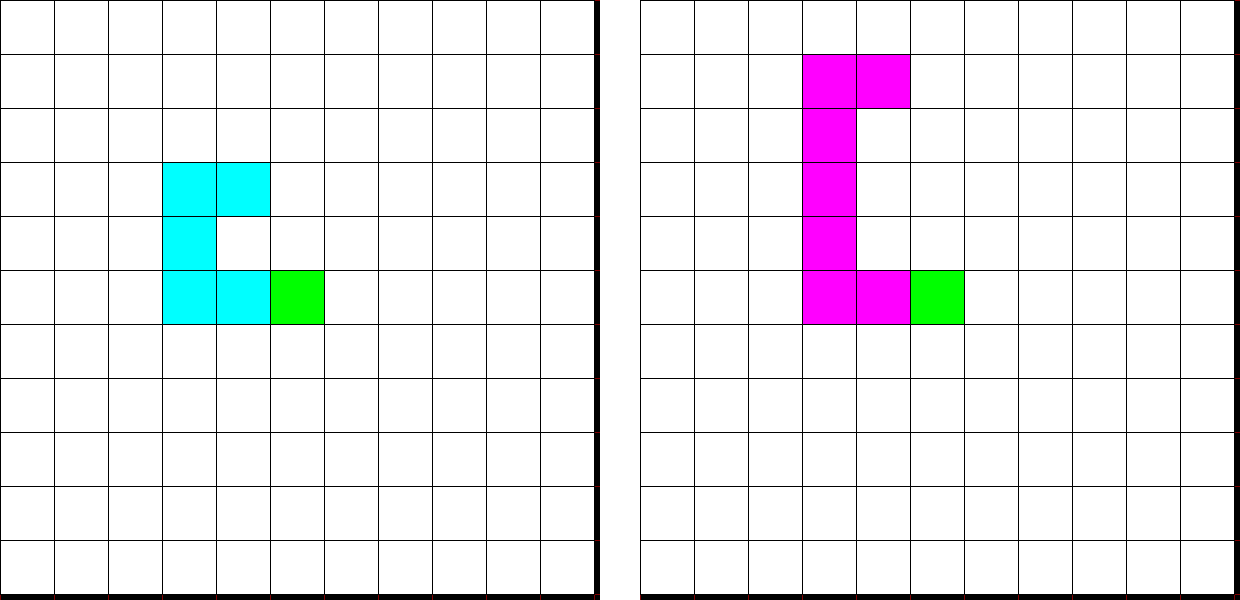
We get the two following tracjectories. One in the agent’s envrionment in blue and one in the predictive environment. They are not the same however they are close one to another.

Optimisation

Now that we have generated a trajectory we need to find the optimal sequence of action such that the trajectory is minimizing the cost function. They are different way of doing so and a lot of ongoing research focuses on this question. We present here a simple Optimisation for linear time invarient (LTI) systems and quadratic cost. For those that are unfamiliar with LTIs it is a system where the dynamic equations are of the following form:

\[\boldsymbol{x}_{t+1} = \boldsymbol{A}*\boldsymbol{x}_{t} + \boldsymbol{B}*\boldsymbol{u}_{t}\]

A quadratic cost cost is a cost where the action depend term has the following form

\[c(\boldsymbol{x}_{t}, \boldsymbol{u}_{t}) = q(\boldsymbol{x}) + \boldsymbol{u}_{t}^T * \boldsymbol{Q} * \boldsymbol{u}_{t}\]

Note: Bold symbols in lower case indicate a vector and bold symbols in upper case indicate a Matrix.

Now that we have a trajectory and a cost function, we can find the cost of a trajectory. This is simply achieved by summing over the cost at every step.

\[c(H) = \sum_{i=t}^{t+\tau} c(x_{i}, u_{i})\]

And as you can see, this function is quadratic w.r.t to the action sequence. This means that this is a convex function and we can find it’s minimum by taking its derivative and setting it to 0. The sequence of state \(\boldsymbol{X} = \{\boldsymbol{x}_{t},\, \boldsymbol{x}_{t+1},\, \boldsymbol{x}_{t+1},\, ... ,\,\boldsymbol{x}_{t+\tau}\}\) is built by recursively applying the predictive model.

Controller.

Now we have all the building blocks to create a MPC algorithm.

MPC algorithm.

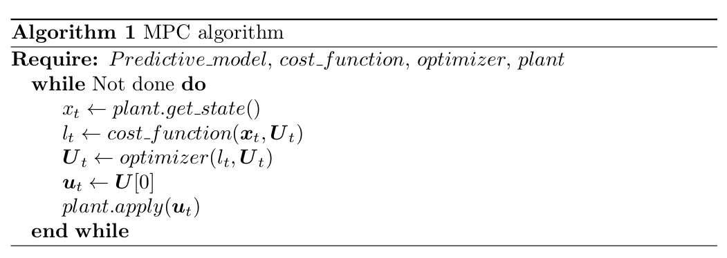
So as showed in the algorithm the entire process is as follows:

1. Get the new state of the agent.
2. Compute the cost of the current action sequence by “rolling out” the predictive model.
3. Optimize the action sequence using the optimizer.
4. Send the first action of the action sequence to the system.
5. Start again from point 1.

This will effectively make MPC a feeback controller.

Conclusion.

You should now have a clearer and better understanding of MPC. This powerfull algorithm is ganing a lot of interest over the recent years. There is a lot a research going on on non-linear MPC controller. In some following blog posts we will review a sampling-based non-linear MPC called MPPI into more details.